pytorch를 이용한 1 ~ 5층 까지의 신경망 구성해보기.
MNIST DataSet Load
jupyter notebook에서 MNIST데이터를 받으려 했지만, 실행이 되지않아 colab에서 MNIST 데이터를 받는 방식으로 했다.
import gzip
import os
import sys
import struct
import numpy as np

import pandas as pd
import time

import torch
from torch import nn
from torch import optim
from torch.utils.data import TensorDataset
from torch.utils.data import DataLoader

# visualization
from matplotlib.legend_handler import HandlerLine2D
import matplotlib.pyplot as plt
%matplotlib inline


import gc

def read_image(fi):
    magic, n, rows, columns = struct.unpack(">IIII", fi.read(16))
    assert magic == 0x00000803
    assert rows == 28
    assert columns == 28
    rawbuffer = fi.read()
    assert len(rawbuffer) == n * rows * columns
    rawdata = np.frombuffer(rawbuffer, dtype='>u1', count=n*rows*columns)
    return rawdata.reshape(n, rows, columns).astype(np.float32) / 255.0

def read_label(fi):
    magic, n = struct.unpack(">II", fi.read(8))
    assert magic == 0x00000801
    rawbuffer = fi.read()
    assert len(rawbuffer) == n
    return np.frombuffer(rawbuffer, dtype='>u1', count=n)

if __name__ == '__main__':
    os.system('wget -N http://yann.lecun.com/exdb/mnist/train-images-idx3-ubyte.gz')
    os.system('wget -N http://yann.lecun.com/exdb/mnist/train-labels-idx1-ubyte.gz')
    os.system('wget -N http://yann.lecun.com/exdb/mnist/t10k-images-idx3-ubyte.gz')
    os.system('wget -N http://yann.lecun.com/exdb/mnist/t10k-labels-idx1-ubyte.gz')

    np.savez_compressed(
        'mnist',
        train_x=read_image(gzip.open('train-images-idx3-ubyte.gz', 'rb')),
        train_y=read_label(gzip.open('train-labels-idx1-ubyte.gz', 'rb')),
        test_x=read_image(gzip.open('t10k-images-idx3-ubyte.gz', 'rb')),
        test_y=read_label(gzip.open('t10k-labels-idx1-ubyte.gz', 'rb'))
    )
data = np.load('mnist.npz')
x_train = data['train_x']
y_train = data['train_y']
x_test = data['test_x']
y_test = data['test_y']
Data Reshape
이 방식으로 데이터를 받으면 (60000, 28, 28) 형태의 데이터로 로드되기 때문에 x 데이터들을 1차원 벡터형태로 펴준다.
# x_train.shaep : (60000, 28, 28) -> (60000, 784)
# x_test.shape : (10000, 28, 28) -> (10000, 784)
x_train = x_train.reshape((60000, 784))
x_test = x_test.reshape((10000, 784))
to pytorch tensor
pytorch를 이용해 신경망을 구성할것이기 때문에 torch.tensor로 변경해준다.
이유는 모르겠지만 y데이터의 형태를 long으로 바꾸지 않으면 선형 계산 과정에서 예외가 뜨며 실행이 되지않는다.
def preprocess(x, y):
    return x.to(dev, dtype=torch.float), y.to(dev, dtype=torch.long)


class WrappedDataLoader:
    def __init__(self, dl, func):
        self.dl = dl
        self.func = func

    def __len__(self):
        return len(self.dl)

    def __iter__(self):
        batches = iter(self.dl)
        for b in batches:
            yield (self.func(*b))

def get_data(train_ds, valid_ds, bs):
    return (
        DataLoader(train_ds, batch_size=bs, shuffle=True),
        DataLoader(valid_ds, batch_size=bs * 2),
    )
print(torch.cuda.is_available())
dev = torch.device("cuda") if torch.cuda.is_available() else torch.device("cpu")
true
import torch
x_train, y_train, x_test, y_test = map(
    torch.tensor, (x_train, y_train, x_test, y_test)
)
batch_size = 4096
train_ds = TensorDataset(X_train, y_train)
valid_ds = TensorDataset(X_valid, y_valid)
train_dl, valid_dl = get_data(train_ds, valid_ds, batch_size)
train_dl = WrappedDataLoader(train_dl, preprocess)
valid_dl = WrappedDataLoader(valid_dl, preprocess)
DNN implement
MyModule
인자로 layer의 갯수를 받을 수 있도록 nn.ModuleList()를 이용해 설계를 하였다.
def fc_layer(size_in, size_out, keep_prob, xavier=True):
    linear = nn.Linear(size_in, size_out)
    if xavier :
        torch.nn.init.xavier_uniform_(linear.weight)
    layer = nn.Sequential(
        linear,
        nn.BatchNorm1d(size_out),
        nn.ReLU(),
        nn.Dropout(p = 1 - keep_prob)
    )
    return layer

class MyModule(nn.Module):
    def __init__(self, input = 784, layer = [10], keep_prob = 1, xavier = True):
        super().__init__()
        self.log_softmax = nn.LogSoftmax()
        self.linears = nn.ModuleList()

        self.input = input

        for output in layer :
            self.linears.append(fc_layer(self.input, output, keep_prob, xavier))
            self.input = output
        self.linears.append(fc_layer(self.input, 10, keep_prob, xavier))

    def forward(self, x):
        for linear in self.linears :
            # apply dropout
            x = linear(x)
        # output layer
        x = self.log_softmax(x)
        return x
def accuracy(out, yb):
    preds = torch.argmax(out, dim=1)
    return (preds == yb).float().mean()

# model, optim 설정
def get_model(layer = [10], lr = 0.01):
    model = MyModule(layer)
    return model, optim.SGD(model.parameters(), lr=lr)

'''
test 데이터와, train 데이터일때의 구별을 하기위해 opt = None으로 설정
test 데이터에서 쓸데없이 parameter 업데이트가 되지 않도록 하기 위해서
'''
def loss_batch(model, loss_func, xb, yb, opt=None):
    loss = loss_func(model(xb), yb)
    if opt is not None:
        loss.backward()
        opt.step()
        opt.zero_grad()
    return loss.item()

'''
fit 함수
x_train, y_train으로 학습을 끝낸 후
train, test의 정확도를 출력
'''
def fit(epochs, model, loss_func, opt, train_dl, test_dl):
    start = time.time()
    train_loss = []
    for epoch in range(epochs):
        model.train()
        for xb, yb in train_dl:
            loss = loss_batch(model, loss_func, xb, yb, opt)
        train_loss.append(loss)
        if (epoch + 1) % 10 == 0:
            print('{} epoch is done'.format(epoch + 1))
    print('train accuracy : ', accuracy(model(x_train), y_train))
    print('test accuracy : ', accuracy(model(x_test), y_test))
    print("cost time :", time.time() - start)
    return train_loss
# Cross entropy loss func
loss_func = F.cross_entropy

epochs = 200
lr = 0.05
Layer 갯수와 accuracy 비교
Layer의 갯수와 accuracy 관계를 살펴보겠다.
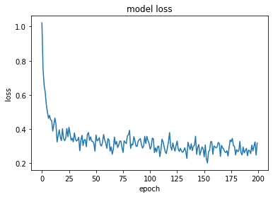
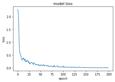
Layer : 1
model, opt = get_model(layer = [512], lr = lr)
train_loss = fit(epochs, model, loss_func, opt, train_dl, test_dl)
10 epoch is done
20 epoch is done
30 epoch is done
40 epoch is done
50 epoch is done
60 epoch is done
70 epoch is done
80 epoch is done
90 epoch is done
100 epoch is done
110 epoch is done
120 epoch is done
130 epoch is done
140 epoch is done
150 epoch is done
160 epoch is done
170 epoch is done
180 epoch is done
190 epoch is done
200 epoch is done
train accuracy :  tensor(0.9222)
test accuracy :  tensor(0.9223)
cost time : 104.36
plt.plot(train_loss)
plt.title('model loss')
plt.ylabel('loss')
plt.xlabel('epoch')
plt.show()
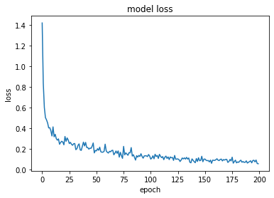
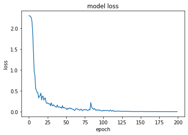
Layer : 2
model, opt = get_model(layer = [512, 256], lr = lr)
train_loss = fit(epochs, model, loss_func, opt, train_dl, test_dl)
10 epoch is done
20 epoch is done
30 epoch is done
40 epoch is done
50 epoch is done
60 epoch is done
70 epoch is done
80 epoch is done
90 epoch is done
100 epoch is done
110 epoch is done
120 epoch is done
130 epoch is done
140 epoch is done
150 epoch is done
160 epoch is done
170 epoch is done
180 epoch is done
190 epoch is done
200 epoch is done
train accuracy :  tensor(0.9813)
test accuracy :  tensor(0.9726)
cost time : 415.87
plt.plot(train_loss)
plt.title('model loss')
plt.ylabel('loss')
plt.xlabel('epoch')
plt.show()
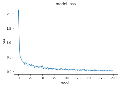
Layer : 3
model, opt = get_model(layer = [512, 256, 128], lr = lr)
train_loss = fit(epochs, model, loss_func, opt, train_dl, test_dl)
10 epoch is done
20 epoch is done
30 epoch is done
40 epoch is done
50 epoch is done
60 epoch is done
70 epoch is done
80 epoch is done
90 epoch is done
100 epoch is done
110 epoch is done
120 epoch is done
130 epoch is done
140 epoch is done
150 epoch is done
160 epoch is done
170 epoch is done
180 epoch is done
190 epoch is done
200 epoch is done
train accuracy :  tensor(0.9946)
test accuracy :  tensor(0.9786)
cost time : 578.93
plt.plot(train_loss)
plt.title('model loss')
plt.ylabel('loss')
plt.xlabel('epoch')
plt.show()
Layer : 4
model, opt = get_model(layer = [512, 256, 128, 64], lr = lr)
train_loss = fit(epochs, model, loss_func, opt, train_dl, test_dl)
10 epoch is done
20 epoch is done
30 epoch is done
40 epoch is done
50 epoch is done
60 epoch is done
70 epoch is done
80 epoch is done
90 epoch is done
100 epoch is done
110 epoch is done
120 epoch is done
130 epoch is done
140 epoch is done
150 epoch is done
160 epoch is done
170 epoch is done
180 epoch is done
190 epoch is done
200 epoch is done
train accuracy :  tensor(0.9995)
test accuracy :  tensor(0.9795)
cost time : 622.08
plt.plot(train_loss)
plt.title('model loss')
plt.ylabel('loss')
plt.xlabel('epoch')
plt.show()
Layer : 5
model, opt = get_model(layer = [512, 256, 128, 64, 32], lr = lr)
train_loss = fit(epochs, model, loss_func, opt, train_dl, test_dl)
10 epoch is done
20 epoch is done
30 epoch is done
40 epoch is done
50 epoch is done
60 epoch is done
70 epoch is done
80 epoch is done
90 epoch is done
100 epoch is done
110 epoch is done
120 epoch is done
130 epoch is done
140 epoch is done
150 epoch is done
160 epoch is done
170 epoch is done
180 epoch is done
190 epoch is done
200 epoch is done
train accuracy :  tensor(1.0000)
test accuracy :  tensor(0.9787)
cost time : 633.75
plt.plot(train_loss)
plt.title('model loss')
plt.ylabel('loss')
plt.xlabel('epoch')
plt.show()
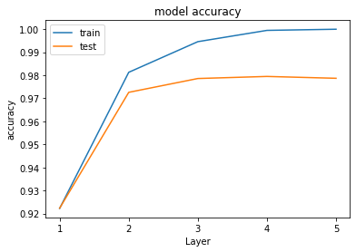
종합적인 비교
각 layer 노드가 많아 시간이 오래걸려 하이퍼파라미터 튜닝을 많이 못해봤지만 이것저것 건들여 보면서 느낀것이 확실이 Layer가 많을수록 성능이 좋아질 확률이 있다. 대신 Layer가 많으면 epoch를 더 많이 주어야한다.
- epoch : 100 일 때, Layer 5의 accuracy 성능 (0.9420, 0.9361)
- epoch : 200 일 때, Layer 5의 accuracy 성능 (1.0000, 0.9787)
정확도가 1이 나올 수 있다는 것이 참 놀랍다.
- 하지만 오버피팅임을 알 수 있다.
확실이 Machine Learning 모델(SVM, Logistic Regression 등등)로 돌렸을 때보다 성능이 많이 좋은것이 체감이되고, torch.nn 모듈 사용으로 인해 코드가 정말 간결해졌다.
train_accuracy = [0.9222, 0.9813, 0.9946, 0.9995, 1.0000]
test_accuracy = [0.9223, 0.9726, 0.9786, 0.9795, 0.9787]
x = [1, 2, 3, 4, 5]
# summarize history for accuracy
plt.plot(x, train_accuracy)
plt.plot(x, test_accuracy)
plt.title('model accuracy')
plt.ylabel('accuracy')
plt.xlabel('Layer')
plt.xticks(x)
plt.legend(['train', 'test'], loc='upper left')
plt.show()