- feature decision
- Drop features
- Target
- Categorical features
- Numercial features
- 이상치처리가 필요한 features
- CHOLE Data
- 이상치, 결측치 처리완료
- Feature Create
feature decision
Drop features
HCHK_YEARIDV_IDHCHK_OE_INSPEC_YNCRS_YNTTH_MSS_YNODT_TRB_YNWSDM_DIS_YNTTR_YNDATA_STD__DT
Target
당뇨(2) :
126 <= BLDS전당뇨(1) :
100 <= BLDS < 126정상(0) :
BLDS < 100
Categorical features
SEXSIDOHEAR_LEFTHEAR_RIGHTSMK_STAT_TYPE_CDDRK_YN
Numercial features
AGE_GROUPHEIGHTWEIGHTBMIWAISTSIGHT_LEFTSIGHT_RIGHTOLIG_PROTE_CDBP_HIGHBP_LWSTTOT_CHOLETRIGLYCERIDEHDL_CHOLELDL_CHOLEHMGCREATININESGOT_ASTSGPT_ALTGAMMA_GTP
# data analysis and wrangling
import pandas as pd
import numpy as np
import random as rnd
import scipy.stats as stats
from scipy.stats.mstats import winsorize
pd.set_option('display.max_columns', 100)
pd.set_option('display.max_rows', 100)


# visualization
import missingno as msno
import seaborn as sns
import matplotlib.pyplot as plt
%matplotlib inline

# ignore warnings
import warnings
warnings.filterwarnings(action='ignore')


# machine learning
from sklearn.linear_model import LinearRegression
from sklearn.linear_model import LogisticRegression
from sklearn.svm import SVC, LinearSVC
from sklearn.ensemble import RandomForestClassifier
from sklearn.neighbors import KNeighborsClassifier
from sklearn.naive_bayes import GaussianNB
from sklearn.linear_model import Perceptron
from sklearn.linear_model import SGDClassifier
from sklearn.tree import DecisionTreeClassifier
from sklearn.model_selection import train_test_split
data_2017 = pd.read_csv('./NHIS_2017_2018_100m/NHIS_OPEN_GJ_2017_100.csv')
data_2018 = pd.read_csv('./NHIS_2017_2018_100m/NHIS_OPEN_GJ_2018_100.csv')
df = pd.concat([data_2017,data_2018])
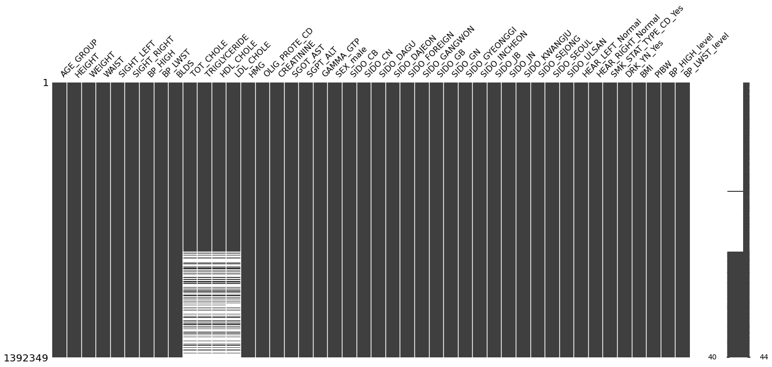
Drop features
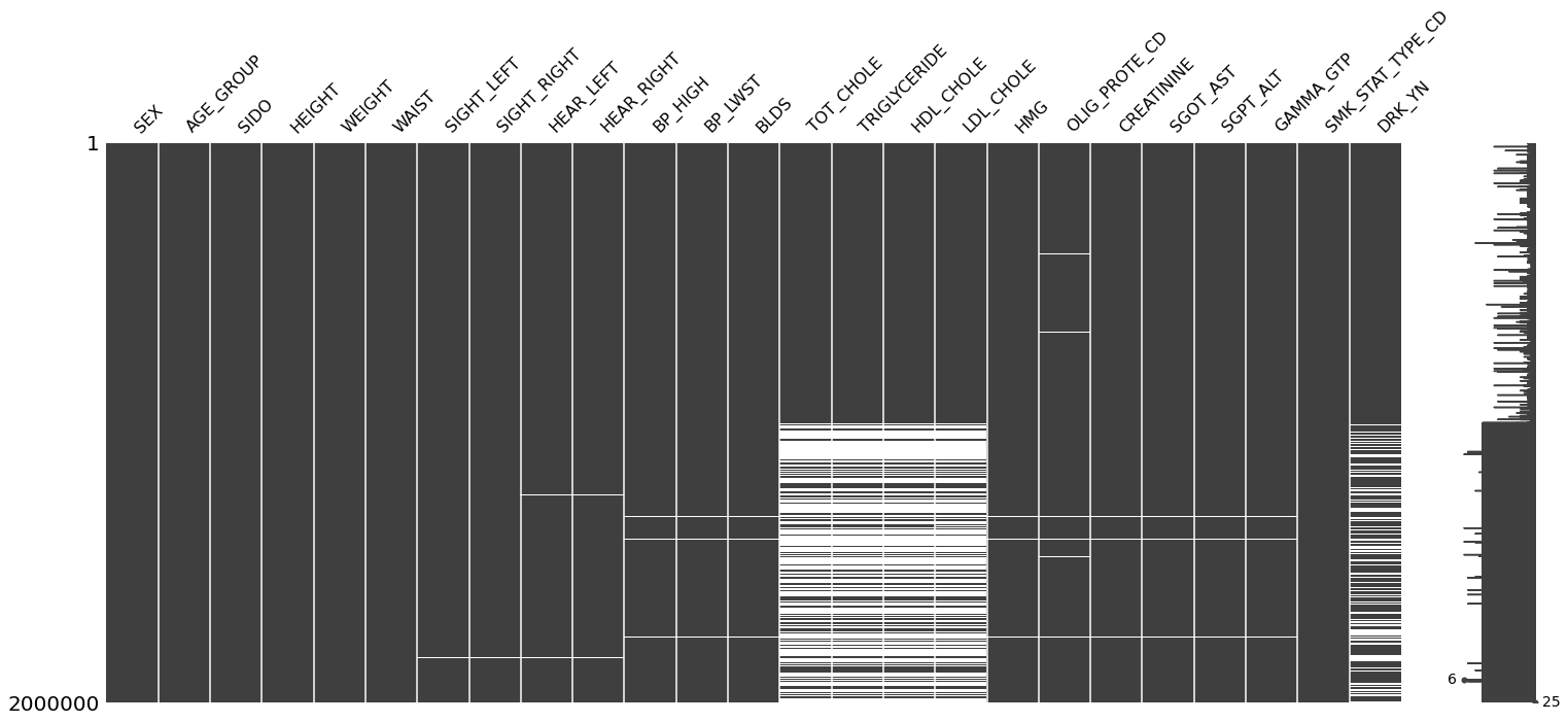
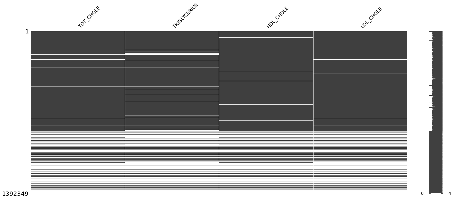
필요없는 feature들을 삭제하고 결측치 분포를 보니 'TOT_CHOLE', 'TRIGLYCERIDE', 'HDL_CHOLE', 'LDL_CHOLE'의 결측치가 가장 많고, 또한 결측치가 서로 몰려있는 것을 확인할 수 있다.
drop_cols = ['HCHK_YEAR', 'IDV_ID', 'HCHK_OE_INSPEC_YN', 'CRS_YN', 'TTH_MSS_YN', 'ODT_TRB_YN', 'TTR_YN', 'WSDM_DIS_YN', 'DATA_STD__DT']
df.drop(drop_cols, axis = 1, inplace = True)
# error시 : sudo conda install missingno
msno.matrix(df)
plt.show()
Target
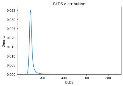
당뇨병의 무서운점은 당뇨병 자체가 아니라 그로인해 발생하는 합병증 때문인다. 따라서 당뇨병은 조기진단이 매우 중요한 질병이다. 따라서 정상, 전당뇨, 당뇨 환자를 예측하는 Target을 설정한다.
전당뇨 정보
당뇨(2) :
126 <= BLDS전당뇨(1) :
100 <= BLDS < 126정상(0) :
BLDS < 100
sns.kdeplot(df.BLDS)
plt.title("BLDS distribution")
plt.show()
p = len(df[df['BLDS'] >= 126])
print('[공복혈당 126 이상]당뇨환자 수치 : {}%'.format(100 * p / len(df)))
p = len(df[(100 <= df['BLDS']) & (df['BLDS'] < 126)])
print('[공복혈당 100 이상 126 미만]전 당뇨환자 수치 : {}%'.format(100 * p / len(df)))
p = len(df[df['BLDS'] < 100])
print('[공복혈당 100 미만]정상인 수치 : {}%'.format(100 * p / len(df)))
[공복혈당 126 이상]당뇨환자 수치 : 7.795%
[공복혈당 100 이상 126 미만]전 당뇨환자 수치 : 30.21825%
[공복혈당 100 미만]정상인 수치 : 61.6889%
df.loc[ df['BLDS'] < 100, 'BLDS'] = 0
df.loc[(100 <= df['BLDS']) & (df['BLDS'] < 126), 'BLDS'] = 1
df.loc[126 <= df['BLDS'], 'BLDS'] = 2
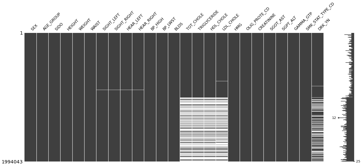
df = df.dropna(subset = ['BLDS'], how = 'any', axis=0)
msno.matrix(df)
plt.show()
print(df.isnull().sum())
SEX                      0
AGE_GROUP                0
SIDO                     0
HEIGHT                   0
WEIGHT                   0
WAIST                  672
SIGHT_LEFT             417
SIGHT_RIGHT            434
HEAR_LEFT              357
HEAR_RIGHT             355
BP_HIGH                 40
BP_LWST                 40
BLDS                     0
TOT_CHOLE           661336
TRIGLYCERIDE        661346
HDL_CHOLE           661347
LDL_CHOLE           671083
HMG                     26
OLIG_PROTE_CD         9274
CREATININE               4
SGOT_AST                 2
SGPT_ALT                 3
GAMMA_GTP                6
SMK_STAT_TYPE_CD       377
DRK_YN              350820
dtype: int64
Categorical features
범주형 데이터들은 모두 one-hot-encoding 해준다
SEXSIDOHEAR_LEFTHEAR_RIGHTSMK_STAT_TYPE_CDDRK_YN
SEX
성비
- 남 : 여 = 1.4 : 1
남성이 여성보다 유병률이 높다
- 남성 : 45%
- 여성 : 30%
mapper = {1 : 'male', 2 : 'female'}
df['SEX'].replace(mapper, inplace=True)
df_ = df[["SEX", "BLDS"]]
df_['BLDS'] = np.where(df_['BLDS'] == 2, 1, df_['BLDS'])
df_.groupby(['SEX'], as_index=False).mean().sort_values(by='BLDS', ascending=False)
| SEX | BLDS | |
|---|---|---|
| 1 | male | 0.443937 |
| 0 | female | 0.309574 |
df['SEX'] = df['SEX'].astype('category')
pd.get_dummies(df['SEX'], drop_first=True)
| male | |
|---|---|
| 0 | 1 |
| 1 | 1 |
| 2 | 1 |
| 3 | 1 |
| 4 | 1 |
| ... | ... |
| 999995 | 0 |
| 999996 | 1 |
| 999997 | 1 |
| 999998 | 1 |
| 999999 | 1 |
1994043 rows × 1 columns
df = pd.get_dummies(df, drop_first=True)
SIDO
식습관 때문인지 지역별로 당뇨 유병률에 차이가 있음을 알 수 있다.
그런데 매뉴얼에 나와있지않은 도시코드(50)가 하나있는데 아마 외국인이 아닌가 싶다
mapper = {11 : 'SEOUL',
          26 : 'BUSAN',
          27 : 'DAGU',
          28 : 'INCHEON',
          29 : 'KWANGJU',
          30 : 'DAJEON',
          31 : 'ULSAN',
          36 : 'SEJONG',
          41 : 'GYEONGGI',
          42 : 'GANGWON',
          43 : 'CB',
          44 : 'CN',
          45 : 'JB',
          46 : 'JN',
          47 : 'GB',
          48 : 'GN',
          49 : 'JEJU',
          50 : 'FOREIGN'}
df['SIDO'].replace(mapper, inplace=True)
df_ = df[["SIDO", "BLDS"]]
df_['BLDS'] = np.where(df_['BLDS'] == 2, 1, df_['BLDS'])
df_[["SIDO", "BLDS"]].groupby(['SIDO'], as_index=False).mean().sort_values(by='BLDS', ascending=False)
| SIDO | BLDS | |
|---|---|---|
| 12 | JN | 0.462556 |
| 13 | KWANGJU | 0.424325 |
| 6 | GANGWON | 0.403643 |
| 0 | BUSAN | 0.402681 |
| 2 | CN | 0.394814 |
| 11 | JB | 0.389559 |
| 8 | GN | 0.389298 |
| 5 | FOREIGN | 0.383460 |
| 7 | GB | 0.382897 |
| 10 | INCHEON | 0.378945 |
| 4 | DAJEON | 0.376976 |
| 9 | GYEONGGI | 0.374150 |
| 1 | CB | 0.370957 |
| 16 | ULSAN | 0.365135 |
| 15 | SEOUL | 0.360828 |
| 3 | DAGU | 0.354118 |
| 14 | SEJONG | 0.349973 |
df['SIDO'] = df['SIDO'].astype('category')
pd.get_dummies(df['SIDO'], drop_first=True)
| CB | CN | DAGU | DAJEON | FOREIGN | GANGWON | GB | GN | GYEONGGI | INCHEON | JB | JN | KWANGJU | SEJONG | SEOUL | ULSAN | |
|---|---|---|---|---|---|---|---|---|---|---|---|---|---|---|---|---|
| 0 | 1 | 0 | 0 | 0 | 0 | 0 | 0 | 0 | 0 | 0 | 0 | 0 | 0 | 0 | 0 | 0 |
| 1 | 0 | 0 | 0 | 0 | 0 | 0 | 0 | 0 | 0 | 0 | 0 | 0 | 0 | 0 | 1 | 0 |
| 2 | 0 | 0 | 0 | 0 | 0 | 0 | 0 | 0 | 1 | 0 | 0 | 0 | 0 | 0 | 0 | 0 |
| 3 | 0 | 0 | 0 | 0 | 0 | 0 | 0 | 1 | 0 | 0 | 0 | 0 | 0 | 0 | 0 | 0 |
| 4 | 0 | 0 | 0 | 1 | 0 | 0 | 0 | 0 | 0 | 0 | 0 | 0 | 0 | 0 | 0 | 0 |
| ... | ... | ... | ... | ... | ... | ... | ... | ... | ... | ... | ... | ... | ... | ... | ... | ... |
| 999995 | 0 | 0 | 0 | 0 | 0 | 0 | 0 | 0 | 1 | 0 | 0 | 0 | 0 | 0 | 0 | 0 |
| 999996 | 0 | 0 | 0 | 0 | 0 | 0 | 0 | 0 | 1 | 0 | 0 | 0 | 0 | 0 | 0 | 0 |
| 999997 | 0 | 0 | 0 | 0 | 0 | 0 | 0 | 0 | 1 | 0 | 0 | 0 | 0 | 0 | 0 | 0 |
| 999998 | 0 | 0 | 0 | 0 | 0 | 0 | 0 | 0 | 1 | 0 | 0 | 0 | 0 | 0 | 0 | 0 |
| 999999 | 0 | 0 | 0 | 0 | 0 | 0 | 1 | 0 | 0 | 0 | 0 | 0 | 0 | 0 | 0 | 0 |
1994043 rows × 16 columns
df = pd.get_dummies(df, drop_first=True)
HEAR_LEFT
왼쪽귀에 이상이 있는 사람은 당뇨병 유병률이 높으므로 결측치(357)를 당뇨병환자를 기준으로 처리한다.
- 당뇨환자 -> DEAF
- 정상인 -> Normal
mapper = {1: 'Normal', 2 : 'DEAF'}
df['HEAR_LEFT'].replace(mapper, inplace=True)
df_ = df[["HEAR_LEFT", "BLDS"]]
df_['BLDS'] = np.where(df_['BLDS'] == 2, 1, df_['BLDS'])
df_[["HEAR_LEFT", "BLDS"]].groupby(['HEAR_LEFT'], as_index=False).mean().sort_values(by='BLDS', ascending=False)
| HEAR_LEFT | BLDS | |
|---|---|---|
| 0 | DEAF | 0.499736 |
| 1 | Normal | 0.377315 |
normal_case = (df['BLDS'] == 1) & (df['HEAR_LEFT'].isnull()) # fill 0
deaf_case = (df['BLDS'] == 0) & (df['HEAR_LEFT'].isnull()) # fill 1
df.loc[normal_case,'HEAR_LEFT'] = df.loc[normal_case,'HEAR_LEFT'].fillna('Normal')
df.loc[deaf_case,'HEAR_LEFT'] = df.loc[deaf_case,'HEAR_LEFT'].fillna('DEAF')
df['HEAR_LEFT'] = df['HEAR_LEFT'].astype('category')
pd.get_dummies(df['HEAR_LEFT'], drop_first=True)
| Normal | |
|---|---|
| 0 | 1 |
| 1 | 1 |
| 2 | 1 |
| 3 | 1 |
| 4 | 1 |
| ... | ... |
| 999995 | 1 |
| 999996 | 1 |
| 999997 | 1 |
| 999998 | 1 |
| 999999 | 1 |
1994043 rows × 1 columns
df = pd.get_dummies(df, drop_first=True)
HEAR_RIGHT
왼쪽귀에 이상이 있는 사람은 당뇨병 유병률이 높으므로 결측치(355)를 당뇨병환자를 기준으로 처리한다.
- 당뇨환자 -> DEAF
- 정상인 -> Normal
mapper = {1: 'Normal', 2 : 'DEAF'}
df['HEAR_RIGHT'].replace(mapper, inplace=True)
df_ = df[["HEAR_RIGHT", "BLDS"]]
df_['BLDS'] = np.where(df_['BLDS'] == 2, 1, df_['BLDS'])
df_[["HEAR_RIGHT", "BLDS"]].groupby(['HEAR_RIGHT'], as_index=False).mean().sort_values(by='BLDS', ascending=False)
| HEAR_RIGHT | BLDS | |
|---|---|---|
| 0 | DEAF | 0.501281 |
| 1 | Normal | 0.377412 |
normal_case = (df['BLDS'] == 1) & (df['HEAR_RIGHT'].isnull()) # fill 0
deaf_case = (df['BLDS'] == 0) & (df['HEAR_RIGHT'].isnull()) # fill 1
df.loc[normal_case,'HEAR_RIGHT'] = df.loc[normal_case,'HEAR_RIGHT'].fillna('Normal')
df.loc[deaf_case,'HEAR_RIGHT'] = df.loc[deaf_case,'HEAR_RIGHT'].fillna('DEAF')
df['HEAR_RIGHT'] = df['HEAR_RIGHT'].astype('category')
pd.get_dummies(df['HEAR_RIGHT'], drop_first=True)
| Normal | |
|---|---|
| 0 | 1 |
| 1 | 1 |
| 2 | 1 |
| 3 | 1 |
| 4 | 1 |
| ... | ... |
| 999995 | 1 |
| 999996 | 1 |
| 999997 | 1 |
| 999998 | 1 |
| 999999 | 1 |
1994043 rows × 1 columns
df = pd.get_dummies(df, drop_first=True)
SMK_STAT_TYPE_CD
흡연자는 당뇨병 유병률이 높으므로 결측치(377)를 당뇨병환자를 기준으로 처리한다.
- 당뇨환자 -> Yes
- 정상인 -> No
mapper = {1: 'No', 2 : 'No', 3: 'Yes'}
df['SMK_STAT_TYPE_CD'].replace(mapper, inplace=True)
df_ = df[["SMK_STAT_TYPE_CD", "BLDS"]]
df_['BLDS'] = np.where(df_['BLDS'] == 2, 1, df_['BLDS'])
df_[["SMK_STAT_TYPE_CD", "BLDS"]].groupby(['SMK_STAT_TYPE_CD'], as_index=False).mean().sort_values(by='BLDS', ascending=False)
| SMK_STAT_TYPE_CD | BLDS | |
|---|---|---|
| 1 | Yes | 0.428212 |
| 0 | No | 0.368393 |
smoke = (df['BLDS'] == 1) & (df['SMK_STAT_TYPE_CD'].isnull()) # fill 0
non_smoke = (df['BLDS'] == 0) & (df['SMK_STAT_TYPE_CD'].isnull()) # fill 1
df.loc[smoke,'SMK_STAT_TYPE_CD'] = df.loc[smoke,'SMK_STAT_TYPE_CD'].fillna('Yes')
df.loc[non_smoke,'SMK_STAT_TYPE_CD'] = df.loc[non_smoke,'SMK_STAT_TYPE_CD'].fillna('No')
df['SMK_STAT_TYPE_CD'] = df['SMK_STAT_TYPE_CD'].astype('category')
pd.get_dummies(df['SMK_STAT_TYPE_CD'], drop_first=True)
| Yes | |
|---|---|
| 0 | 0 |
| 1 | 1 |
| 2 | 0 |
| 3 | 0 |
| 4 | 0 |
| ... | ... |
| 999995 | 0 |
| 999996 | 0 |
| 999997 | 0 |
| 999998 | 0 |
| 999999 | 0 |
1994043 rows × 1 columns
df = pd.get_dummies(df, drop_first=True)
DRK_YN
음주는 당뇨병을 악화시키지만, 음주 여부는 당뇨 유병률에 큰 차이를 보이지 않기 때문에 결측치(350820) 개의 행은 삭제 시킨다.
mapper = {1: 'Yes', 0 : 'No'}
df['DRK_YN'].replace(mapper, inplace=True)
df_ = df[["DRK_YN", "BLDS"]]
df_['BLDS'] = np.where(df_['BLDS'] == 2, 1, df_['BLDS'])
df_[["DRK_YN", "BLDS"]].groupby(['DRK_YN'], as_index=False).mean().sort_values(by='BLDS', ascending=False)
| DRK_YN | BLDS | |
|---|---|---|
| 1 | Yes | 0.387572 |
| 0 | No | 0.359463 |
# 결측치 행 삭제
df = df.dropna(subset = ['DRK_YN'], how = 'any', axis=0)
df['DRK_YN'] = df['DRK_YN'].astype('category')
pd.get_dummies(df['DRK_YN'], drop_first=True)
| Yes | |
|---|---|
| 0 | 1 |
| 1 | 0 |
| 2 | 0 |
| 3 | 0 |
| 4 | 0 |
| ... | ... |
| 999993 | 1 |
| 999994 | 1 |
| 999996 | 1 |
| 999997 | 1 |
| 999999 | 1 |
1643223 rows × 1 columns
df = pd.get_dummies(df, drop_first=True)
Numercial features
결측치, 이상치를 적절히 전처리해준다.
AGE_GROUPHEIGHTWEIGHTBMIWAISTSIGHT_LEFTSIGHT_RIGHTOLIG_PROTE_CDBP_HIGHBP_LWSTTOT_CHOLETRIGLYCERIDEHDL_CHOLELDL_CHOLEHMGCREATININESGOT_ASTSGPT_ALTGAMMA_GTP
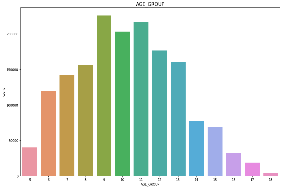
AGE_GROUP
Discrete Numercial type
결측치, 이상치는 없다
plt.figure(figsize=(15,10))
sns.countplot(df['AGE_GROUP'])
plt.title("AGE_GROUP",fontsize=15)
plt.show()
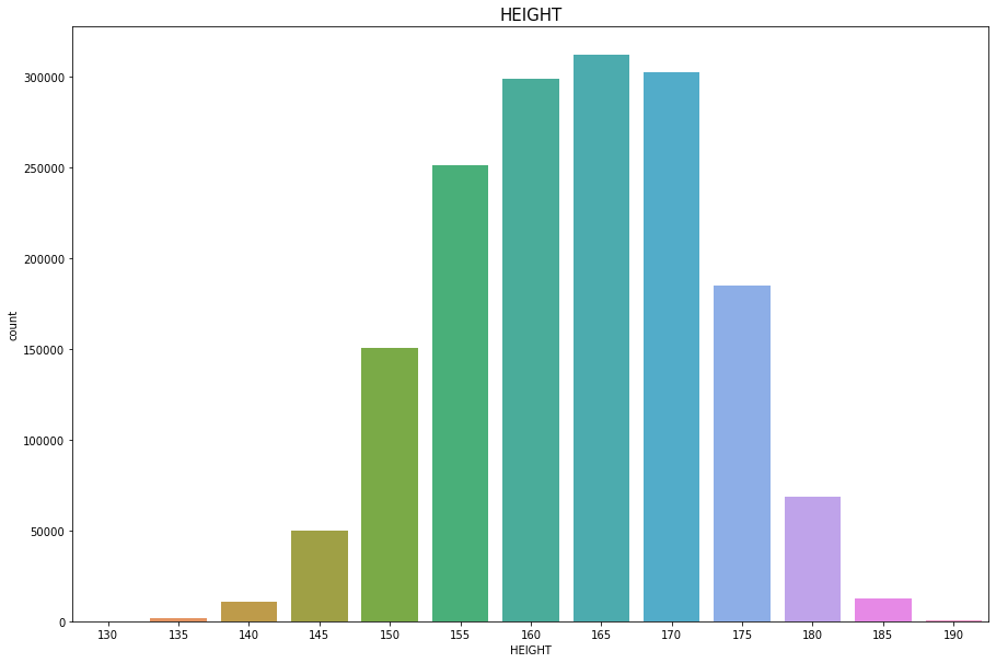
HEIGHT
Discrete Numercial type
결측치, 이상치는 없다
plt.figure(figsize=(15,10))
sns.countplot(df['HEIGHT'])
plt.title("HEIGHT",fontsize=15)
plt.show()
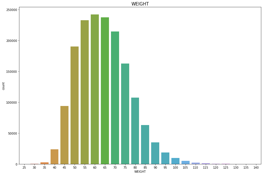
WEIGHT
Discrete Numercial type
결측치, 이상치는 없다
plt.figure(figsize=(15,10))
sns.countplot(df['WEIGHT'])
plt.title("WEIGHT",fontsize=15)
plt.show()
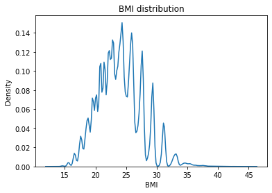
BMI(체질량지수)
Feature Create
Continuous Numercial type
df['WEIGHT'] / (df['HEIGHT']/100)**2
df['BMI'] = df['WEIGHT'] / (df['HEIGHT']/100)**2
sns.kdeplot(df.BMI)
plt.title("BMI distribution")
plt.show()
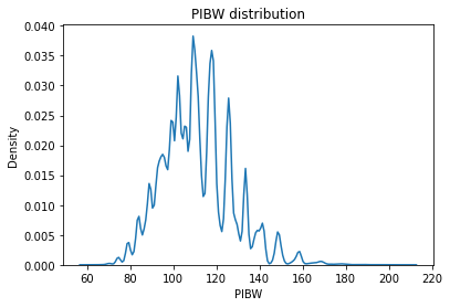
PIBW(체질량지수)
Feature Create
Continous Numercial type
표준 체중과 비교해 얼마나 차이가 나는지 확인하는 지표
- (0, 90%) : 저체중
- (90%, 110%) : 정상체중
- (110%, 120%) : 과체중
- (120%,~) : 비만
PIBW = 100 * 측정체중 / 표준체중
df['PIBW'] = np.where(df['SEX_male'] == 1, (100*df['WEIGHT'])/(22*(df['HEIGHT']/100)**2), (100*df['WEIGHT'])/(21*(df['HEIGHT']/100)**2))
sns.kdeplot(df.PIBW)
plt.title("PIBW distribution")
plt.show()
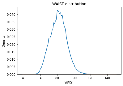
WAIST
Continous Numercial type
결측치(394)와 양측에 이상치가 존재한다.
허리둘레가 999cm 인사람 58명
허리둘레가 45cm가 안되는 사람 15명
허리둘레 45cm면 웬만한 마른 아이돌 허리둘레보다 얇은 길이인데 이보다 훨씬 얇은 사람들이 있다.
이상치 및 결측치를 [‘HEIGHT’, ‘WEIGHT’, ‘BMI’, ‘PIBW’]를 이용해 Linear Regression으로 채워준다.
# 900이상의 허리둘레는 잘못 기입된 값이므로 이상치로 처리한다.
df['WAIST'] = np.where(df['WAIST']>900, np.nan, df['WAIST'])
# 40cm미만의 허리둘레는 잘못 기입된 값이므로 이상치로 처리한다.
df['WAIST'] = np.where(df['WAIST']<40, np.nan, df['WAIST'])
sns.kdeplot(df.WAIST)
plt.title("WAIST distribution")
plt.show()
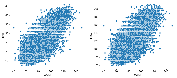
BMI, PIBW 와 WAIST의 상관관계
각 0.8, 0.75로 높은 상관성을 띈다.
fig, (ax1,ax2) = plt.subplots(ncols=2)
fig.set_size_inches(12, 5)
sns.scatterplot(data=df, y="BMI", x = 'WAIST', ax=ax1)
sns.scatterplot(data=df, y="PIBW", x = 'WAIST', ax=ax2)
print(df[['PIBW', 'BMI','WAIST']].corr())
           PIBW       BMI     WAIST
PIBW   1.000000  0.987789  0.756360
BMI    0.987789  1.000000  0.807472
WAIST  0.756360  0.807472  1.000000
Linear Regression으로 WAIST 결측치 및 이상치 채우기
72% 정도의 정확성을 가진 Linear Regression 모델로 WAIST결측치를 채운 새로운 WAIST_LR feature를 생성하고 기존 WAIST는 삭제
df_copy = df[df['WAIST'].notnull()][['BMI', 'PIBW', 'WAIST', 'HEIGHT', 'WEIGHT']]
X_train, X_test, y_train, y_test = train_test_split(df_copy[['BMI', 'PIBW', 'HEIGHT', 'WEIGHT']],
                                                    df_copy['WAIST'], random_state=42)
lr = LinearRegression()
lr.fit(X_train, y_train)
lr.score(X_test, y_test)
0.7271066870154038
df['WAIST_pred'] = lr.predict(df[['BMI','PIBW', 'HEIGHT', 'WEIGHT']])
df['WAIST'] = np.where(df['WAIST']>0, df['WAIST'], df['WAIST_pred'])
sns.kdeplot(df.WAIST)
plt.title("WAIST distribution")
plt.show()

# 임시 feature WAIST_pred drop
drop_cols = ['WAIST_pred']
df.drop(drop_cols, axis = 1, inplace = True)
SIGHT_LEFT
Discrete Numercial type
이상치는 없지만 실명(9.9)을 0으로 바꾸어준다.
결측치(273)은 수가 적으니 평균시력(1)로 채워준다.
# 실명 9.9 -> 0
df['SIGHT_LEFT'] = np.where(df['SIGHT_LEFT']>2.5, 0, df['SIGHT_LEFT'])
plt.figure(figsize=(15,10))
sns.countplot(df['SIGHT_LEFT'])
plt.title("SIGHT_LEFT",fontsize=15)
plt.show()
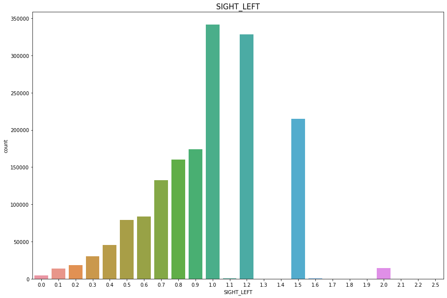
df['SIGHT_LEFT'].fillna(1, inplace = True)
SIGHT_RIGHT
Discrete Numercial type
이상치는 없지만 실명(9.9)을 0으로 바꾸어준다.
결측치(283)은 수가 적으니 평균시력(1)로 채워준다.
# 실명 9.9 -> 0
df['SIGHT_RIGHT'] = np.where(df['SIGHT_RIGHT']>2.5, 0, df['SIGHT_RIGHT'])
plt.figure(figsize=(15,10))
sns.countplot(df['SIGHT_RIGHT'])
plt.title("SIGHT_RIGHT",fontsize=15)
plt.show()
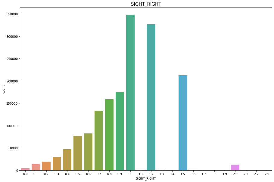
df['SIGHT_RIGHT'].fillna(1, inplace = True)
OLIG_PROTE_CD
Discrete Numercial type
결측치(7009)
데이터상으로 요단백수치와 당뇨는 관계가 없다.
- 요단백수치 2이상인 사람중 당뇨 유병률 : 5%
멱분포를 따르는것같다. 압도적으로 1이 많기 때문에 결측치 7009개를 1로 채워준다
plt.figure(figsize=(15,10))
sns.countplot(df['OLIG_PROTE_CD'])
plt.title("OLIG_PROTE_CD",fontsize=15)
plt.show()
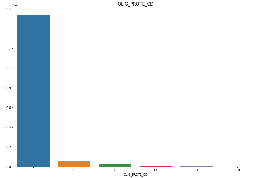
df['OLIG_PROTE_CD'].fillna(1, inplace = True)
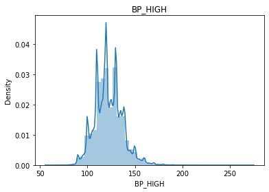
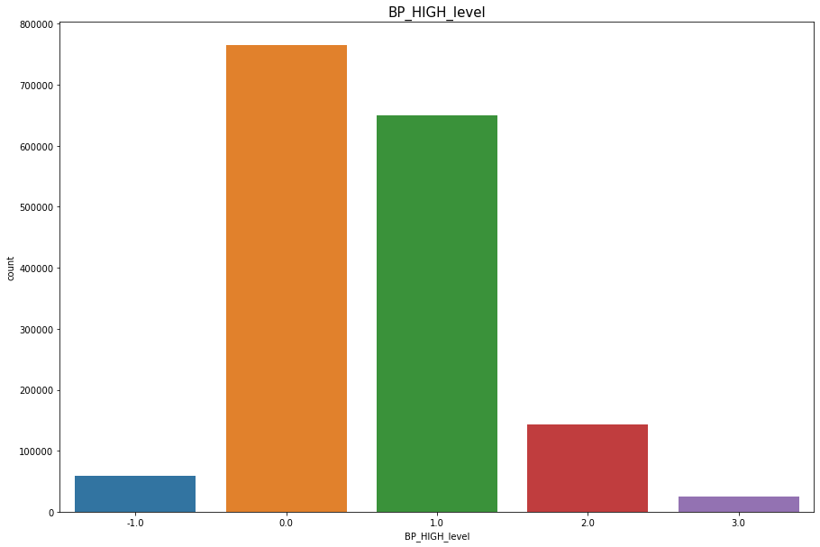
BP_HIGH
Continous Numercial type 결측치(25)수가 적으므로 drop 해준다.
수축기 혈압이 10의 배수인 부근에 값이 몰려있는것을 발견할 수 있는데 이는 혈압 측정자가 반올림을 하여 10단위 구간에 값들이 몰려있는것 같다.
- 0 ~ 99 : 저혈압(-1)
- 100~120 : 정상(0)
- 121~139 : 전고혈압(1)
- 140~159 : 1단계 고혈압(2)
- 160 ~ : 2단계 고혈압(3)
df = df.dropna(subset = ['BP_HIGH'], how = 'any', axis=0)
sns.distplot(df.BP_HIGH)
plt.title("BP_HIGH")
plt.show()
df['BP_HIGH_level'] = np.where(160 <= df['BP_HIGH'], 3, df['BP_HIGH'])
df['BP_HIGH_level'] = np.where((140<=df['BP_HIGH']) & (df['BP_HIGH']<160), 2, df['BP_HIGH_level'])
df['BP_HIGH_level'] = np.where((121<=df['BP_HIGH']) & (df['BP_HIGH']<140), 1, df['BP_HIGH_level'])
df['BP_HIGH_level'] = np.where((100<=df['BP_HIGH']) & (df['BP_HIGH']<=120), 0, df['BP_HIGH_level'])
df['BP_HIGH_level'] = np.where((df['BP_HIGH'].min()<=df['BP_HIGH']) & (df['BP_HIGH']<100), -1, df['BP_HIGH_level'])
plt.figure(figsize=(15,10))
sns.countplot(df['BP_HIGH_level'])
plt.title("BP_HIGH_level",fontsize=15)
plt.show()
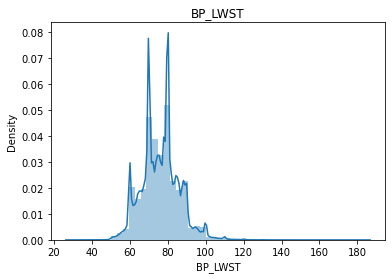
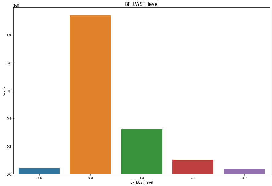
BP_LWST
Continous Numercial type 결측치(1)수가 적으므로 drop 해준다.
이완기 혈압이 10의 배수인 부근에 값이 몰려있는것을 발견할 수 있는데 이는 혈압 측정자가 반올림을 하여 10단위 구간에 값들이 몰려있는것 같다.
- 0 ~ 59 : 저혈압(-1)
- 60~80 : 정상(0)
- 81~89 : 전고혈압(1)
- 90~99 : 1단계 고혈압(2)
- 100 ~ : 2단계 고혈압(3)
df = df.dropna(subset = ['BP_LWST'], how = 'any', axis=0)
sns.distplot(df.BP_LWST)
plt.title("BP_LWST")
plt.show()
df['BP_LWST_level'] = np.where(100 <= df['BP_LWST'], 3, df['BP_LWST'])
df['BP_LWST_level'] = np.where((90<=df['BP_LWST']) & (df['BP_LWST']<100), 2, df['BP_LWST_level'])
df['BP_LWST_level'] = np.where((81<=df['BP_LWST']) & (df['BP_LWST']<90), 1, df['BP_LWST_level'])
df['BP_LWST_level'] = np.where((60<=df['BP_LWST']) & (df['BP_LWST']<=80), 0, df['BP_LWST_level'])
df['BP_LWST_level'] = np.where((df['BP_LWST'].min()<=df['BP_LWST']) & (df['BP_LWST']<60), -1, df['BP_LWST_level'])
plt.figure(figsize=(15,10))
sns.countplot(df['BP_LWST_level'])
plt.title("BP_LWST_level",fontsize=15)
plt.show()
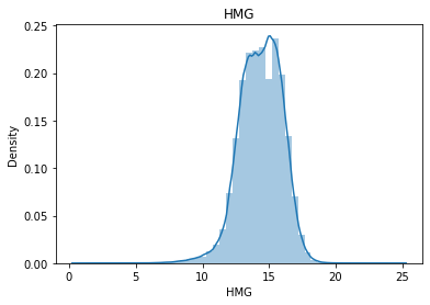
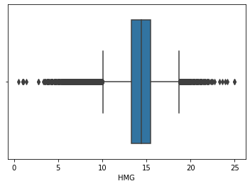
HMG
Continous Numercial type
결측치(24)수가 적으므로 drop 해준다.
정규분포를 띄지만 약간의 이상치가 존재한다.
df = df.dropna(subset = ['HMG'], how = 'any', axis=0)
sns.distplot(df.HMG)
plt.title("HMG")
plt.show()
sns.boxplot(data=df, x='HMG')
<AxesSubplot:xlabel='HMG'>
이상치처리가 필요한 features
- CREATININE
- SGOT_AST
- SGPT_ALT
- GAMMA_GTP
4개의 feature들은 모두 공통적으로 극단적인 큰값들이 분포해있는것으로 보아 잘못기입되거나, 오류가아닌 실제로 건강이 안좋아서 나온 수치들로 보여진다. 하지만 이렇게 극단적인 값들을 그대로 가지고 training 시켰을 때, 결과물이 outlier에 의해 치우져질 가능성이 매우크기 때문에 outlier처리를 해야한다.
우선 4개의 feature 결측치의 수는 적으므로 drop 해준다
4개의 feature의 outlier 분포를 확인한 결과, outlier들은 특정 사람에게 몰려있는 것이아닌 random하게 분포되어있음을 확인했다.
# 4개의 feature 결측치 제거
df = df.dropna(subset = ['CREATININE', 'SGOT_AST', 'SGPT_ALT', 'GAMMA_GTP'], how = 'any', axis=0)
outlier = df[['CREATININE', 'SGOT_AST', 'SGPT_ALT', 'GAMMA_GTP']].copy()
for col in outlier :
  q1 = outlier[col].quantile(0.25)
  q3 = outlier[col].quantile(0.75)
  iqr = q3 - q1
  lower_bound = q1 - (iqr * 1.5)
  upper_bound = q3 + (iqr * 1.5)
  print('{}\'s upper bound : {}, lower bount : {}'.format(col, round(upper_bound, 2), round(lower_bound, 2)))
  outlier[col] = np.where(outlier[col] > upper_bound, np.nan, outlier[col])
  outlier[col] = np.where(outlier[col] < lower_bound, np.nan, outlier[col])
msno.matrix(outlier)
plt.show()

outlier.isnull().sum()
print(outlier.isnull().sum())
print('-'*30)
print('전체 이상치 개수 :', len(outlier) - len(outlier.dropna()))
CREATININE's upper bound : 1.45, lower bount : 0.25
SGOT_AST's upper bound : 44.0, lower bount : 4.0
SGPT_ALT's upper bound : 52.5, lower bount : -7.5
GAMMA_GTP's upper bound : 81.0, lower bount : -23.0
CREATININE     12069
SGOT_AST       95285
SGPT_ALT      119253
GAMMA_GTP     149083
dtype: int64
------------------------------
전체 이상치 개수 : 250811
fig, axes = plt.subplots(nrows = 3, ncols=4, figsize=(18, 12))
for i, col in enumerate(outlier) :
  sns.kdeplot(df[col], ax = axes[0][i])
  sns.countplot(outlier[col],ax = axes[1][i])
  sns.boxplot(data=outlier, x=col, orient="v", ax = axes[2][i])
plt.setp(axes.flat, xlabel=None, ylabel=None)
pad = 5
rows = ['include outlier', 'exclude outlier', 'exclude outlier boxplot']
for ax, row in zip(axes[:,0], rows):
    ax.annotate(row, xy=(0, 0.5), xytext=(-ax.yaxis.labelpad - pad, 0),
                xycoords=ax.yaxis.label, textcoords='offset points',
                size='large', ha='right', va='center')

fig.tight_layout()
plt.show()
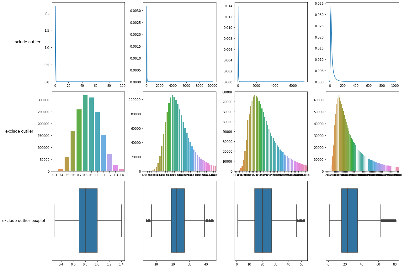
1행 : 기존 데이터 분포
2행 : 이상치 제거한 데이터 분포
3행 : 이상치 제거한 boxplot
# delete outlier
outlier = ['CREATININE', 'SGOT_AST', 'SGPT_ALT', 'GAMMA_GTP']
for col in outlier :
  q1 = df[col].quantile(0.25)
  q3 = df[col].quantile(0.75)
  iqr = q3 - q1
  lower_bound = q1 - (iqr * 1.5)
  upper_bound = q3 + (iqr * 1.5)
  df[col] = np.where(df[col] > upper_bound, np.nan, df[col])
  df[col] = np.where(df[col] < lower_bound, np.nan, df[col])

df = df.dropna(subset = outlier, how = 'any', axis=0)
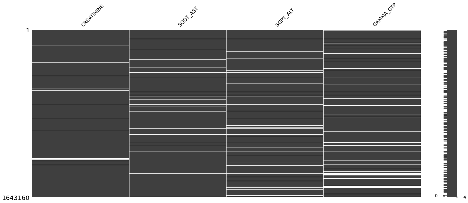
중간점검
결측치가 가장많이 몰려있는 콜레스테롤 관련 features들
- TOT_CHOLE
- TRIGLYCERIDE
- HDL_CHOLE
- LDL_CHOLE
을 제외한 데이터 전처리를 끝냈다.
msno.matrix(df)
plt.show()
print(df.isnull().sum())
AGE_GROUP                    0
HEIGHT                       0
WEIGHT                       0
WAIST                        0
SIGHT_LEFT                   0
SIGHT_RIGHT                  0
BP_HIGH                      0
BP_LWST                      0
BLDS                         0
TOT_CHOLE               369826
TRIGLYCERIDE            369832
HDL_CHOLE               369831
LDL_CHOLE               374327
HMG                          0
OLIG_PROTE_CD                0
CREATININE                   0
SGOT_AST                     0
SGPT_ALT                     0
GAMMA_GTP                    0
SEX_male                     0
SIDO_CB                      0
SIDO_CN                      0
SIDO_DAGU                    0
SIDO_DAJEON                  0
SIDO_FOREIGN                 0
SIDO_GANGWON                 0
SIDO_GB                      0
SIDO_GN                      0
SIDO_GYEONGGI                0
SIDO_INCHEON                 0
SIDO_JB                      0
SIDO_JN                      0
SIDO_KWANGJU                 0
SIDO_SEJONG                  0
SIDO_SEOUL                   0
SIDO_ULSAN                   0
HEAR_LEFT_Normal             0
HEAR_RIGHT_Normal            0
SMK_STAT_TYPE_CD_Yes         0
DRK_YN_Yes                   0
BMI                          0
PIBW                         0
BP_HIGH_level                0
BP_LWST_level                0
dtype: int64
CHOLE Data
- TOT_CHOLE
- TRIGLYCERIDE
- HDL_CHOLE
- LDL_CHOLE
outlier = df[['TOT_CHOLE', 'TRIGLYCERIDE', 'HDL_CHOLE', 'LDL_CHOLE']].copy()
a = len(outlier.dropna())
for col in outlier :
  q1 = outlier[col].quantile(0.25)
  q3 = outlier[col].quantile(0.75)
  iqr = q3 - q1
  lower_bound = q1 - (iqr * 1.5)
  upper_bound = q3 + (iqr * 1.5)
  print('{}\'s upper bound : {}, lower bount : {}'.format(col, round(upper_bound, 2), round(lower_bound, 2)))
  outlier[col] = np.where(outlier[col] > upper_bound, np.nan, outlier[col])
  outlier[col] = np.where(outlier[col] < lower_bound, np.nan, outlier[col])
msno.matrix(outlier)
plt.show()

outlier.isnull().sum()
print(outlier.isnull().sum())
print('-'*30)
print('전체 이상치 및 outlier 개수 :', len(outlier) - len(outlier.dropna()))
TOT_CHOLE's upper bound : 291.5, lower bount : 95.5
TRIGLYCERIDE's upper bound : 266.0, lower bount : -46.0
HDL_CHOLE's upper bound : 94.5, lower bount : 18.5
LDL_CHOLE's upper bound : 200.0, lower bount : 24.0
TOT_CHOLE       381142
TRIGLYCERIDE    422080
HDL_CHOLE       388140
LDL_CHOLE       385875
dtype: int64
------------------------------
전체 이상치 및 outlier 개수 : 454367
fig, axes = plt.subplots(nrows = 3, ncols=4, figsize=(18, 12))
for i, col in enumerate(outlier) :
  sns.kdeplot(df[col], ax = axes[0][i])
  sns.countplot(outlier[col],ax = axes[1][i])
  sns.boxplot(data=outlier, x=col, orient="v", ax = axes[2][i])
plt.setp(axes.flat, xlabel=None, ylabel=None)

pad = 5
rows = ['include outlier', 'exclude outlier', 'exclude outlier boxplot']
for ax, row in zip(axes[:,0], rows):
    ax.annotate(row, xy=(0, 0.5), xytext=(-ax.yaxis.labelpad - pad, 0),
                xycoords=ax.yaxis.label, textcoords='offset points',
                size='large', ha='right', va='center')

fig.tight_layout()
plt.show()
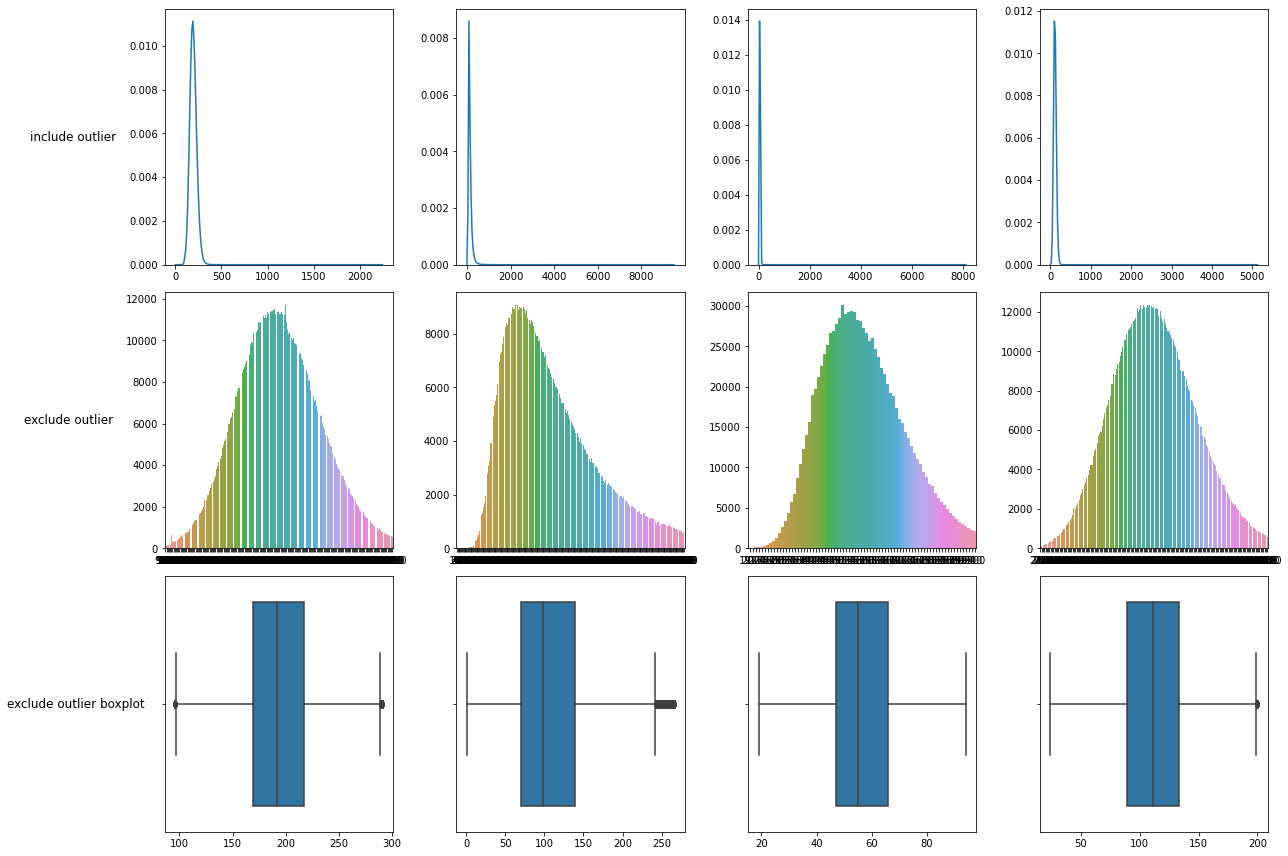
1행 : 기존 데이터 분포
2행 : 이상치 제거한 데이터 분포
3행 : 이상치 제거한 boxplot
# 이상치 제거
cols = ['TOT_CHOLE', 'TRIGLYCERIDE', 'HDL_CHOLE', 'LDL_CHOLE']
for col in cols :
  q1 = df[col].quantile(0.25)
  q3 = df[col].quantile(0.75)
  iqr = q3 - q1
  lower_bound = q1 - (iqr * 1.5)
  upper_bound = q3 + (iqr * 1.5)
  df = df[(lower_bound<=df[col]) & (df[col] <= upper_bound) | (df[col].isnull())]
countinous = ['AGE_GROUP', 'HEIGHT', 'WEIGHT', 'WAIST', 'SIGHT_LEFT',
'SIGHT_RIGHT', 'BP_HIGH', 'BP_LWST', 'BLDS', 'TOT_CHOLE',
'TRIGLYCERIDE', 'HDL_CHOLE', 'LDL_CHOLE', 'HMG', 'OLIG_PROTE_CD',
'CREATININE', 'SGOT_AST', 'SGPT_ALT', 'GAMMA_GTP', 'BMI', 'PIBW',
'BP_HIGH_level', 'BP_LWST_level']
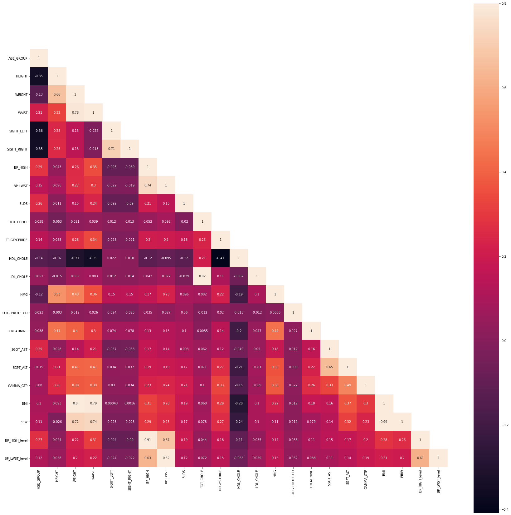
corrMatt = df[countinous].corr()
mask = np.array(corrMatt)
mask[np.tril_indices_from(mask)] = False
f,ax = plt.subplots(figsize=(30, 30))
#sns.heatmap(corrMatt, annot=True, linewidths=.5, fmt= '.1f',ax=ax)
sns.heatmap(corrMatt, mask=mask,vmax=.8, square=True,annot=True, ax = ax)
<AxesSubplot:>
Fill Nan by Regression
Linear Regression 모델링을 통해 결측치를 채워본다.
from sklearn.linear_model import LinearRegression, Ridge, Lasso, ElasticNet
from sklearn.preprocessing import StandardScaler


data = df.copy()
data.dropna(inplace = True)
y_tot = data['TOT_CHOLE']
y_tri = data['TRIGLYCERIDE']
y_hdl = data['HDL_CHOLE']
y_ldl = data['LDL_CHOLE']

drop_cols = ['TOT_CHOLE', 'TRIGLYCERIDE', 'HDL_CHOLE', 'LDL_CHOLE', 'BLDS']
data.drop(drop_cols, axis = 1, inplace = True)
Linear Regression Train & Predict
예측할 4개의 feature과 Target을 제외한 나머지 feature들로 Linear Regression을 시행한 결과 MSE, score이 터무니없이 작게 나와서 예측치로 결측치를 채울 수 없다는 결론을 내렸다. 따라서 결측치는 삭제처리한다.
X_train, X_test, y_tot_train, y_tot_test = train_test_split(data, y_tot, test_size = 0.3, random_state=42)
X_train, X_test, y_tri_train, y_tri_test = train_test_split(data, y_tri, test_size = 0.3, random_state=42)
X_train, X_test, y_hdl_train, y_hdl_test = train_test_split(data, y_hdl, test_size = 0.3, random_state=42)
X_train, X_test, y_ldl_train, y_ldl_test = train_test_split(data, y_ldl, test_size = 0.3, random_state=42)

sc = StandardScaler().fit(X_train)
X_train_sc = sc.transform(X_train)
X_test_sc = sc.transform(X_test)
model_tot = LinearRegression()
model_tot.fit(X_train_sc, y_tot_train)
print("TOT score : ",model_tot.score(X_test_sc, y_tot_test))
y_pred = model_tot.predict(X_test_sc)
print("TOT MSE : ", sum((y_tot_test - y_pred)**2) / len(y_tot_test))
TOT score :  0.05576215500393267
TOT MSE :  1113.3989897779566
model_tri = LinearRegression()
model_tri.fit(X_train_sc, y_tri_train)
print("TRI score : ",model_tri.score(X_test_sc, y_tri_test))
y_pred = model_tri.predict(X_test_sc)
print("TRI MSE : ", sum((y_tri_test - y_pred)**2) / len(y_tri_test))
TRI score :  0.20016898079679968
TRI MSE :  2092.9693749041735
model_hdl = LinearRegression()
model_hdl.fit(X_train_sc, y_hdl_train)
print("HDL score : ",model_hdl.score(X_test_sc, y_hdl_test))
y_pred = model_hdl.predict(X_test_sc)
print("HDL MSE : ", sum((y_hdl_test - y_pred)**2) / len(y_hdl_test))
HDL score :  0.1983517184445205
HDL MSE :  143.9153872584845
model_ldl = LinearRegression()
model_ldl.fit(X_train_sc, y_ldl_train)
print("LDL score : ",model_ldl.score(X_test_sc, y_ldl_test))
y_pred = model_ldl.predict(X_test_sc)
print("LDL MSE : ", sum((y_ldl_test - y_pred)**2) / len(y_ldl_test))
LDL score :  0.041472068147774266
LDL MSE :  949.2267775426899
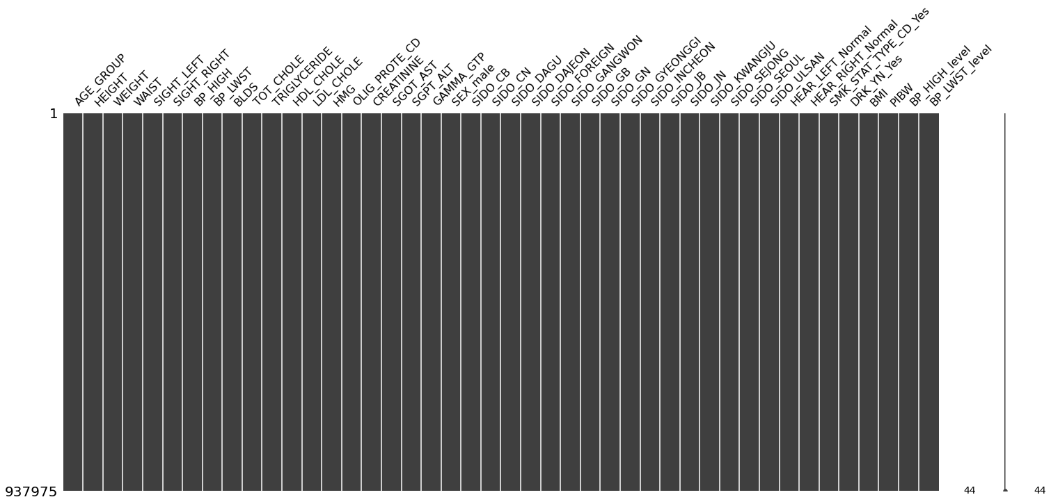
df.dropna(inplace = True)
msno.matrix(df)
plt.show()
df.describe()
| AGE_GROUP | HEIGHT | WEIGHT | WAIST | SIGHT_LEFT | SIGHT_RIGHT | BP_HIGH | BP_LWST | BLDS | TOT_CHOLE | TRIGLYCERIDE | HDL_CHOLE | LDL_CHOLE | HMG | OLIG_PROTE_CD | CREATININE | SGOT_AST | SGPT_ALT | GAMMA_GTP | SEX_male | SIDO_CB | SIDO_CN | SIDO_DAGU | SIDO_DAJEON | SIDO_FOREIGN | SIDO_GANGWON | SIDO_GB | SIDO_GN | SIDO_GYEONGGI | SIDO_INCHEON | SIDO_JB | SIDO_JN | SIDO_KWANGJU | SIDO_SEJONG | SIDO_SEOUL | SIDO_ULSAN | HEAR_LEFT_Normal | HEAR_RIGHT_Normal | SMK_STAT_TYPE_CD_Yes | DRK_YN_Yes | BMI | PIBW | BP_HIGH_level | BP_LWST_level | |
|---|---|---|---|---|---|---|---|---|---|---|---|---|---|---|---|---|---|---|---|---|---|---|---|---|---|---|---|---|---|---|---|---|---|---|---|---|---|---|---|---|---|---|---|---|
| count | 937975.000000 | 937975.000000 | 937975.000000 | 937975.000000 | 937975.000000 | 937975.000000 | 937975.000000 | 937975.000000 | 937975.000000 | 937975.000000 | 937975.000000 | 937975.000000 | 937975.000000 | 937975.000000 | 937975.000000 | 937975.000000 | 937975.000000 | 937975.000000 | 937975.000000 | 937975.000000 | 937975.000000 | 937975.000000 | 937975.000000 | 937975.000000 | 937975.000000 | 937975.000000 | 937975.000000 | 937975.000000 | 937975.000000 | 937975.000000 | 937975.000000 | 937975.000000 | 937975.000000 | 937975.000000 | 937975.000000 | 937975.000000 | 937975.000000 | 937975.000000 | 937975.000000 | 937975.000000 | 937975.000000 | 937975.000000 | 937975.000000 | 937975.000000 |
| mean | 10.517616 | 162.002399 | 62.181599 | 80.212072 | 0.950041 | 0.947671 | 121.454282 | 75.357764 | 0.403228 | 191.829651 | 109.303008 | 57.447467 | 112.449188 | 14.125549 | 1.078551 | 0.841988 | 22.653508 | 20.599382 | 25.501897 | 0.505338 | 0.033069 | 0.041271 | 0.047271 | 0.030269 | 0.010303 | 0.029905 | 0.053449 | 0.066947 | 0.248925 | 0.057672 | 0.035787 | 0.035373 | 0.027682 | 0.004433 | 0.184352 | 0.024929 | 0.968739 | 0.969776 | 0.194926 | 0.551999 | 23.588539 | 109.680289 | 0.533975 | 0.303479 |
| std | 2.837100 | 9.229756 | 11.750765 | 9.191787 | 0.344178 | 0.342207 | 14.283575 | 9.665989 | 0.600539 | 34.335348 | 51.149954 | 13.406158 | 31.477233 | 1.552392 | 0.385756 | 0.190751 | 6.076824 | 9.101093 | 14.839650 | 0.499972 | 0.178817 | 0.198916 | 0.212218 | 0.171328 | 0.100980 | 0.170325 | 0.224928 | 0.249931 | 0.432390 | 0.233122 | 0.185758 | 0.184721 | 0.164060 | 0.066433 | 0.387772 | 0.155910 | 0.174022 | 0.171202 | 0.396144 | 0.497289 | 3.339794 | 15.326171 | 0.750506 | 0.685260 |
| min | 5.000000 | 130.000000 | 25.000000 | 40.000000 | 0.000000 | 0.000000 | 63.000000 | 31.000000 | 0.000000 | 96.000000 | 1.000000 | 20.000000 | 24.000000 | 1.000000 | 1.000000 | 0.300000 | 4.000000 | 1.000000 | 1.000000 | 0.000000 | 0.000000 | 0.000000 | 0.000000 | 0.000000 | 0.000000 | 0.000000 | 0.000000 | 0.000000 | 0.000000 | 0.000000 | 0.000000 | 0.000000 | 0.000000 | 0.000000 | 0.000000 | 0.000000 | 0.000000 | 0.000000 | 0.000000 | 0.000000 | 12.486993 | 59.461870 | -1.000000 | -1.000000 |
| 25% | 9.000000 | 155.000000 | 55.000000 | 74.000000 | 0.700000 | 0.700000 | 110.000000 | 70.000000 | 0.000000 | 168.000000 | 70.000000 | 48.000000 | 90.000000 | 13.100000 | 1.000000 | 0.700000 | 18.000000 | 14.000000 | 15.000000 | 0.000000 | 0.000000 | 0.000000 | 0.000000 | 0.000000 | 0.000000 | 0.000000 | 0.000000 | 0.000000 | 0.000000 | 0.000000 | 0.000000 | 0.000000 | 0.000000 | 0.000000 | 0.000000 | 0.000000 | 1.000000 | 1.000000 | 0.000000 | 0.000000 | 21.403092 | 99.103117 | 0.000000 | 0.000000 |
| 50% | 10.000000 | 160.000000 | 60.000000 | 80.000000 | 1.000000 | 1.000000 | 120.000000 | 75.000000 | 0.000000 | 191.000000 | 98.000000 | 56.000000 | 111.000000 | 14.100000 | 1.000000 | 0.800000 | 22.000000 | 19.000000 | 21.000000 | 1.000000 | 0.000000 | 0.000000 | 0.000000 | 0.000000 | 0.000000 | 0.000000 | 0.000000 | 0.000000 | 0.000000 | 0.000000 | 0.000000 | 0.000000 | 0.000000 | 0.000000 | 0.000000 | 0.000000 | 1.000000 | 1.000000 | 0.000000 | 1.000000 | 23.437500 | 109.013428 | 0.000000 | 0.000000 |
| 75% | 13.000000 | 170.000000 | 70.000000 | 86.000000 | 1.200000 | 1.200000 | 130.000000 | 80.000000 | 1.000000 | 215.000000 | 139.000000 | 66.000000 | 134.000000 | 15.300000 | 1.000000 | 1.000000 | 26.000000 | 25.000000 | 32.000000 | 1.000000 | 0.000000 | 0.000000 | 0.000000 | 0.000000 | 0.000000 | 0.000000 | 0.000000 | 0.000000 | 0.000000 | 0.000000 | 0.000000 | 0.000000 | 0.000000 | 0.000000 | 0.000000 | 0.000000 | 1.000000 | 1.000000 | 0.000000 | 1.000000 | 25.711662 | 118.738404 | 1.000000 | 0.000000 |
| max | 18.000000 | 190.000000 | 140.000000 | 145.000000 | 2.500000 | 2.500000 | 273.000000 | 185.000000 | 2.000000 | 291.000000 | 263.000000 | 95.000000 | 200.000000 | 25.000000 | 6.000000 | 1.400000 | 44.000000 | 52.000000 | 81.000000 | 1.000000 | 1.000000 | 1.000000 | 1.000000 | 1.000000 | 1.000000 | 1.000000 | 1.000000 | 1.000000 | 1.000000 | 1.000000 | 1.000000 | 1.000000 | 1.000000 | 1.000000 | 1.000000 | 1.000000 | 1.000000 | 1.000000 | 1.000000 | 1.000000 | 45.714286 | 209.891119 | 3.000000 | 3.000000 |
df.shape
(937975, 46)
이상치, 결측치 처리완료
데이터 변화 :
2000000 x 34->937975 x 46
Feature Create
ABD_FAT
복부비만 수치
허리둘레가 남자 90, 여자 85이상이면 복부비만(1), 정상(0)으로 해준다.
fat = (df['WAIST'] >= 90) & (df['SEX_male'] == 1) | (df['WAIST'] >= 85) & (df['SEX_male'] == 0)
df['ABD_FAT'] = np.where(fat, 1, 0)
GAMMA_GTP_level
2 if GAMMA_GTP >= 200위험, but GAMMA_GTP.max = 811 if (GAMMA_GTP > 63 and SEX_male == 1) or (GAMMA_GTP > 35 and SEX_male == 0)경고0정상
warn = (df['GAMMA_GTP'] > 63) & (df['SEX_male'] == 1) | (df['GAMMA_GTP'] > 35) & (df['SEX_male'] == 0)
df['GAMMA_GTP_level'] = np.where(warn, 1, 0)